AI Investment Cycles, Portfolio Concentration, and the Cost of Being Early
Lessons from Situational Awareness—and what they may tell us about the next phase of AI investing
IMPORTANT DISCLAIMER — PLEASE READ FIRST
This article is an independent educational and research case study. It is not a criticism of Leopold Aschenbrenner, Situational Awareness LP, any investor, any portfolio company, the artificial-intelligence industry, or the broader AI investment cycle. Nothing here alleges misconduct, negligence, manipulation, bad faith, or wrongdoing by any person or organization. The article is not intended to malign anyone, any company, any industry, or any investment objective.
This is also not investment advice, an investment recommendation, a trading strategy, a solicitation, or an investment thesis. It does not recommend buying, selling, shorting, holding, or avoiding any security, fund, sector, or private investment. The illustrative portfolio later in the article is a risk-management thought experiment—not a model portfolio for readers.
All portfolio-construction descriptions, holdings interpretations, risk measures, return figures, benchmark comparisons and related calculations in this article are based on publicly available online information and calculations derived from that information. The underlying information may be incomplete, delayed, inconsistent, revised or incorrect. The calculations, classifications, assumptions and comparisons may therefore also be wrong or inaccurate. They should not be treated as precise portfolio, performance, risk, valuation or attribution measurements.
This article is intentionally a high-level analytical view—not an exact return-versus-risk study and not a reconstruction of what definitively happened inside the portfolio. Its purpose is to consider, from the limited public record, how the disclosed portfolio appeared to compare with broader markets, where its construction may have been vulnerable, and what general lessons the episode may offer. Any numerical result should be read as an approximate analytical illustration rather than a definitive fact about the fund or any investor.
The purpose is narrow: to share my thoughts on the difference between a technology thesis and a portfolio, how concentration, correlation, leverage, liquidity and sector rotation can interact, and what the current AI capital cycle may teach us about portfolio construction. The work relies on delayed public filings, public market prices, company announcements and attributable financial reporting. It cannot reconstruct the fund’s actual daily positions, derivatives, financing, private marks, transaction prices or audited returns.
Initial summary
This post is to share my thoughts on one of the most interesting portfolio events of the current AI cycle.
This is a high-level interpretation built from public filings, online reporting and public market data. It is not intended to provide exact fund returns, exact portfolio exposures or a definitive account of internal events. The numerical comparisons help illustrate scale, direction and portfolio mechanics; they should not be read as precise measurements of the fund’s actual performance or risk.
Leopold Aschenbrenner’s 2024 essay, Situational Awareness: The Decade Ahead, made a bold and in many ways prescient argument: AI would not remain merely a software story. It would become an industrial mobilization involving advanced chips, memory, networking, data centers, electricity, generation, grid equipment and enormous capital spending.
I think that broad insight remains important.
The issue is that a technology thesis, an industry forecast, a company investment and a leveraged portfolio are four different things.
My conclusion from the public evidence is not that “AI was wrong.” It is that a long-duration and probabilistic AI thesis appears to have been expressed through a portfolio that was highly concentrated in one economic factor, highly sensitive to market momentum and financing, partly illiquid, and reportedly supported by substantial leverage.
Concentration determined what could hurt. Leverage determined how much it could hurt. Liquidity determined how much flexibility the portfolio retained.
That distinction matters far beyond one fund. It matters to any investor concentrating in AI chips, power, data centers, neoclouds, memory, application software or private startups. A portfolio can hold many names across many industries and still be one trade.
The longer market record adds an important qualification. AI infrastructure has delivered extraordinary returns: through August 7, 2026, the SMH semiconductor ETF annualized at approximately 34.9% over five years, compared with 15.1% for QQQ and 13.3% for SPY. Broad AI funds also outperformed, but cloud-software exposure lagged badly. The problem was therefore not that the market rejected AI. It was that the strongest historical winners also carried high volatility, large drawdowns and correlations that could rise exactly when financing became scarce.
Highlights
- The March 31, 2026 Form 13F disclosed $3.856 billion of long shares and convertibles, $1.362 billion of call-underlier value, and $8.459 billion of put-underlier value. The total $13.677 billion SEC Column 4 value was not NAV, option premium, delta exposure or gross exposure.
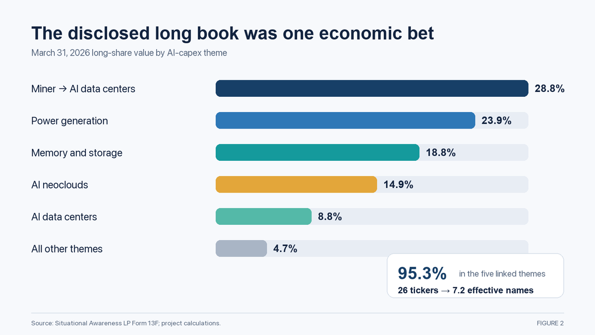
- The disclosed long-share book had 26 tickers, but the top five represented 76.5% of value. Its inverse-HHI “effective number” of positions was only 7.2.
- More than 95% of disclosed long value sat in five linked AI-capex themes: miner-to-data-center conversions, power generation, memory/storage, AI neoclouds and data centers.
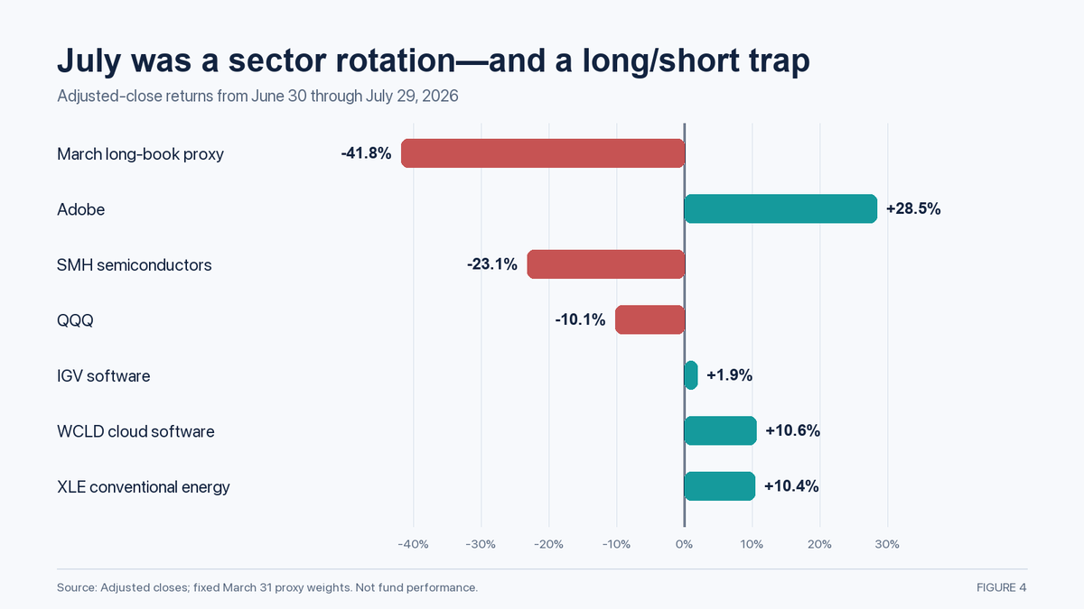
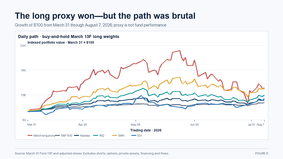
- A fixed-weight proxy based on the March long holdings rose about 111.7% in Q2, then fell 41.8% from June 30 through July 29. This is a proxy, not the fund’s return.
- From March 31 through August 7, the same buy-and-hold long proxy still gained 49.2%, ahead of SPY’s 19.2% and QQQ’s 25.4%, but slightly behind SMH’s 52.0%. Terminal return did not make the path financeable.
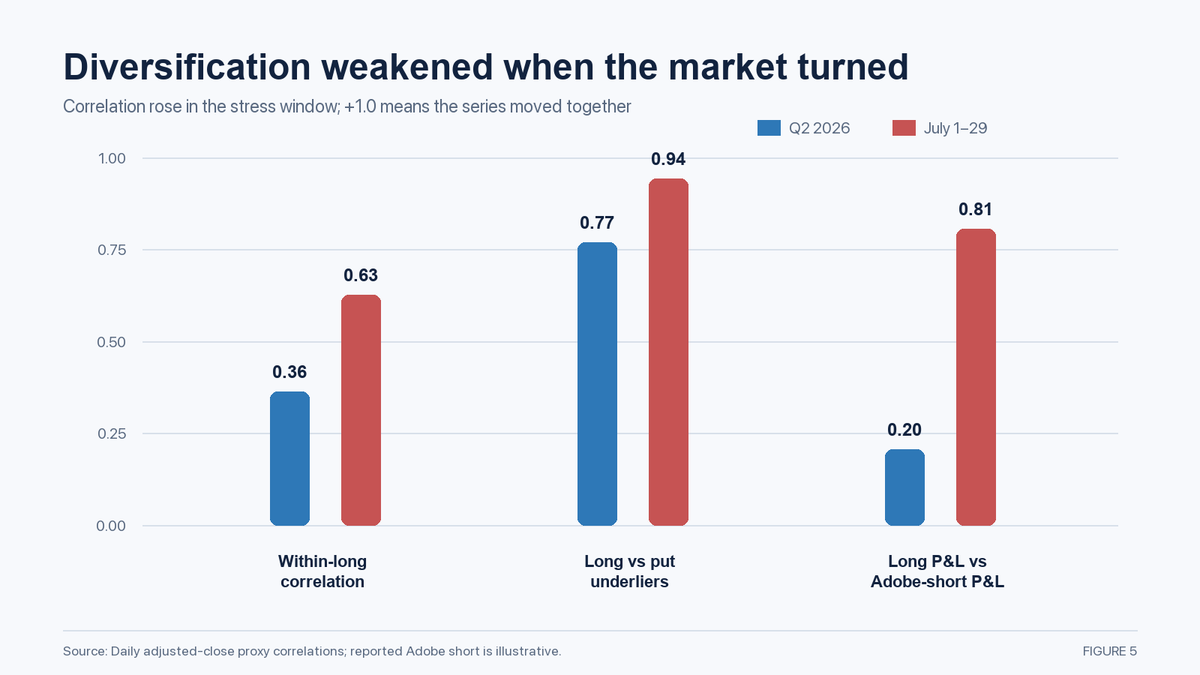
- Weighted within-long correlation rose from 0.36 in Q2 to 0.63 during the July reversal.
- Adobe, identified in financial reporting as one software short, rose 28.5% through July 29. The proxy long-book P&L and an Adobe-short P&L had a +0.81 correlation during the window: they tended to lose together.
- Reporting that the fund borrowed an additional $3–$4 for every $1 of capital implies roughly 4×–5× gross assets to equity before considering exact hedges and netting. At that leverage, an unhedged 20%–25% gross-asset loss can consume the equity.
- The reported 67% July drawdown did not necessarily mean a total wipeout. If a portfolio begins July at 5.39 times its starting-year capital after a 439% return, a 67% decline leaves about 1.78 times starting capital—consistent with subsequent reporting of roughly +80% year to date.
- The main lesson is not “avoid AI infrastructure.” It is: match a 2027–2030 thesis with exposure and liquidity limits that can survive a severe path.
Table of contents
- Why this case matters
- What the original thesis argued
- What public data can and cannot tell us
- What the disclosed portfolio looked like
- The fundamental flaw: the thesis was not the trade
- July’s sector rotation and the long/short problem
- What the longer market record says
- Concentration versus leverage
- What the public evidence does not establish
- Dot-com, housing, currency and LTCM comparisons
- How professional risk teams analyze portfolios
- Private-market AI exposure and the broader capital cycle
- A more survivable AI portfolio framework
- What we may still be missing
- Conclusion
- Methodology and sources
PART 1 | WHY THIS CASE MATTERS
There are two easy but incomplete interpretations of this event.
The first is: “The AI thesis failed.”
The second is: “The portfolio was right, and the market was irrational.”
I do not think either interpretation is sufficient.
AI demand can grow dramatically while an AI security falls. A company can double its revenue while its equity investors lose money. A portfolio can contain the eventual winners and still suffer an unacceptable drawdown. A hedge can be fundamentally sensible and still fail because its strike, expiry, size or timing is wrong. A strategy can be up for the year and still experience a catastrophic institutional loss.
The event is useful because it forces us to separate six questions:
- Is the technology forecast directionally correct?
- Does that forecast produce industry revenue?
- Which companies capture durable profit from that revenue?
- What valuation is already embedded in their securities?
- How are the positions combined and hedged?
- Can the financing survive the path to the forecast?
An investor can be right on question one and wrong on questions three through six.
That is not a criticism of intelligence, conviction or effort. It is the normal difficulty of turning a powerful idea into a portfolio.
The portfolio-risk sequence visible in public data
The public evidence supports a six-link portfolio-risk framework rather than one bad stock call. It does not establish the reasons or decision process behind any specific transaction.

- The thesis identified a genuine industrial bottleneck. Frontier AI appeared likely to require far more chips, memory, data-center capacity and electricity.
- The investment map concentrated on suppliers to that buildout. Multiple sector labels created the appearance of breadth, but the holdings depended on continued AI capital spending, available credit and high utilization.
- Exceptional early returns increased scale. Gains and inflows can increase dollar positions, ownership concentration, confidence and borrowing capacity at precisely the point when exit capacity becomes weakest.
- The short book was not a clean hedge. A “long infrastructure, short software” structure could lose on both sides when infrastructure expectations fell and software companies re-rated or squeezed higher.
- Correlation changed during stress. Positions that looked only moderately related during the rally moved much more closely together during the reversal.
- Leverage increased loss sensitivity and reduced flexibility. At high gross exposure, a relatively modest asset-price decline can consume a large share of equity regardless of the long-term thesis.
This is why the episode is relevant to the broader AI environment. The ecosystem remains unusually dependent on a small number of hyperscalers and frontier labs, large financing commitments, semiconductor and power bottlenecks, and an assumption that demand will arrive quickly enough to absorb the capacity being built. If capex pauses, model efficiency improves faster than usage grows, credit tightens, or applications capture more economics than infrastructure, many apparently different assets can reprice together.
The likely recurrence is not necessarily another identical hedge-fund event. It could appear as a private-credit restructuring, a data-center lease renegotiation, a neocloud refinancing, an ETF crowding event, or a simultaneous de-rating of public suppliers and private marks. The mechanism is the same: a long-duration demand forecast exposed to liabilities or expectations that reprice much faster.
PART 2 | WHAT THE ORIGINAL THESIS ARGUED
Aschenbrenner published Situational Awareness: The Decade Ahead in June 2024. The essay was not a portfolio prospectus. It was a technology, economic and national-security forecast.
Its core sequence was approximately:
AI scaling → much stronger models → intense frontier competition → enormous compute clusters → chips, power and industrial mobilization
The section most directly related to investment was “Racing to the Trillion-Dollar Cluster.” It made unusually concrete estimates.
| Forecast year | Approximate annual AI investment | AI power as share of then-current U.S. electricity | Leading-edge chip requirement |
|---|---|---|---|
| 2024 | $150 billion | 1%–2% | 5%–10% of leading-edge TSMC capacity |
| 2026 | $500 billion | 5% | 25% |
| 2028 | $2 trillion | 20% | 100% |
| 2030 | $8 trillion | 100% | 4× current capacity |
The essay also presented AGI by roughly 2027 as strikingly plausible, expected AI revenue to scale rapidly, and argued that the industrial system would mobilize around data-center clusters, power generation and chip production.
What the thesis saw clearly
Several parts look directionally strong:
- Electricity and interconnection became central AI constraints.
- Memory, storage, networking, cooling and construction matter alongside accelerators.
- Frontier AI-company revenue and private valuations scaled extraordinarily quickly.
- Hyperscalers and new infrastructure providers committed enormous capital.
- Governments increasingly treat advanced AI and semiconductor capacity as strategic.
- Venture investment became historically concentrated around AI.
The International Energy Agency now projects global data-center electricity use to roughly double to 945 TWh by 2030 in its base case. The definitions are different from the essay’s estimates, but the IEA analysis supports the broader point that AI and data centers are becoming material electricity-demand drivers.
Where the investment inference becomes harder
The essay estimated physical quantities more directly than it estimated value capture.
There is a crucial gap between:
- society needing more electricity;
- data centers buying more chips;
- a specific company earning attractive incremental returns;
- its stock outperforming from today’s price;
- and a leveraged owner surviving every drawdown before 2030.
Railways transformed economies, but many railway investors lost money. Fiber-optic capacity made the internet possible, but overbuilding destroyed capital. Housing was genuinely useful, but mortgage structures still created a crisis. A useful asset is not automatically an attractive security at any price and with any financing.
This is the first key lesson: physical necessity does not guarantee investor value capture.
PART 3 | WHAT PUBLIC DATA CAN AND CANNOT TELL US
I used five official Form 13F information tables, from 2025 Q1 through 2026 Q1, later beneficial-ownership filings, company announcements, daily adjusted market prices and attributable financial reporting.
The evidence needs to be separated carefully.
| Evidence category | Example | Confidence and limitation |
|---|---|---|
| Verified regulatory fact | March 2026 Form 13F values and share counts | High confidence for that date and filing scope |
| Verified company announcement | Participation in selected private financings across frontier models, compute infrastructure and semiconductor development | High confidence that an investor participated; usually no fund-level check size, ownership percentage or complete portfolio context |
| Attributable financial reporting | July loss, leverage and reported software shorts | Useful, but not audited here and partly based on confidential sources |
| Quantitative proxy | Fixed March weights applied to later market prices | Reproducible market stress estimate, not actual fund performance |
| General portfolio mechanism | Leverage amplifies gains and losses and can reduce liquidity flexibility | Demonstrated by arithmetic, but not a reconstruction of this fund’s decisions |
| Unknown | The reasons, constraints and decision process behind any specific transaction | Not established by the public data used here |
The most important Form 13F limitation
The official SEC Form 13F guidance explains why the filing cannot be added up into a fund balance sheet.
For a listed option, the filing reports the market value and quantity of the shares underlying the option. It does not report:
- the option premium;
- strike price;
- expiration date;
- delta, gamma, vega or theta;
- whether the position is part of a spread;
- financing or collateral;
- or its realized profit and loss.
The 13F also omits short stock, most foreign securities, private investments, cash, debt, subscriptions, redemptions and complete financing information.
So the March filing’s $8.459 billion of put-underlier value was not necessarily an $8.459 billion short book, hedge book, premium or loss exposure.
That distinction is essential.
PART 4 | WHAT THE DISCLOSED PORTFOLIO LOOKED LIKE
Exposure grew much faster than the effective diversification
| Quarter | Long shares and convertibles | Call-underlier value | Put-underlier value | Top-five long weight | Effective long names |
|---|---|---|---|---|---|
| 2025 Q1 | $0.546B | $0.460B | $0 | 65.6% | 8.6 |
| 2025 Q2 | $1.100B | $0.453B | $0.570B | 85.5% | 5.3 |
| 2025 Q3 | $2.243B | $1.008B | $0.887B | 73.8% | 7.4 |
| 2025 Q4 | $3.914B | $1.594B | $0.009B | 64.9% | 9.1 |
| 2026 Q1 | $3.856B | $1.362B | $8.459B | 76.5% | 7.2 |
The “effective names” measure is the inverse of the Herfindahl concentration index. It answers a useful question: how many equally weighted positions would create similar name concentration?
The answer for March was 7.2—not 26.
The largest disclosed long positions
| Position | March long weight | June 30–July 29 return | Contribution to proxy return |
|---|---|---|---|
| Bloom Energy | 22.8% | -45.9% | -10.5 percentage points |
| Sandisk | 18.8% | -55.3% | -10.4 points |
| CoreWeave | 14.4% | -38.9% | -5.6 points |
| IREN | 10.4% | -35.9% | -3.7 points |
| Core Scientific | 10.1% | -29.2% | -3.0 points |
| Applied Digital | 8.3% | -37.8% | -3.1 points |
Those six names represented 84.8% of the disclosed long-share book and contributed about 36 percentage points of the 41.8% proxy decline.
This is why counting tickers can be misleading.
Bloom Energy, Sandisk, CoreWeave, IREN, Core Scientific and Applied Digital have different products and financial statements. But they can all decline together when the market reduces AI-capex expectations, financing becomes more expensive, high-momentum positions reverse and crowded investors need liquidity.
The economic themes
| Theme | March long weight | Shared risk |
|---|---|---|
| Miner-to-AI/data-center conversions | 28.8% | Financing, construction, dilution, customer demand, crypto sensitivity |
| Power generation | 23.9% | AI-load expectations, project execution, fuel, regulation, duration |
| Memory and storage | 18.8% | Semiconductor cycle, capacity, pricing, inventory |
| AI neoclouds | 14.9% | Utilization, customer concentration, hardware depreciation, debt |
| AI data centers | 8.8% | Power availability, lease commitments, build cost, financing |
| Other | 4.7% | Mixed |
This was not a random collection of speculative stocks. It was a coherent vertical-stack view.
But coherence can become concentration.
PART 5 | THE FUNDAMENTAL FLAW: THE THESIS WAS NOT THE TRADE
The central investment chain was approximately:

Every arrow can break.
1. More compute does not guarantee better infrastructure economics
If supply expands faster than demand, rental pricing and margins fall. If chips become obsolete faster than depreciation schedules assume, owners may report accounting profits but earn weak economic returns. If customers have bargaining power, they capture more of the surplus.
2. Revenue growth does not guarantee equity returns
A stock’s return depends on what was already priced in. A company can deliver extraordinary growth and still underperform if the valuation assumed even more.
This was a central dot-com lesson. The internet transformed the world. That did not make every internet security bought in 1999 a good investment.
3. The AI ecosystem adapts
Algorithmic efficiency, smaller models, distillation, specialized inference hardware, improved utilization and falling cost per task can reduce infrastructure needed per unit of useful work.
Demand may expand enough to offset those gains. It may even expand more than proportionally. But that is a scenario to test, not a certainty to leverage.
4. A vertically diversified portfolio can be factor-concentrated
Chips, power, memory, data centers and neoclouds appear diversified by sector label. In practice they may all be long:
- AI capital spending;
- cheap and available financing;
- high utilization forecasts;
- high equity multiples;
- continued momentum;
- and the absence of overcapacity.
That is one macro bet expressed across multiple income statements.
5. The thesis horizon and portfolio-risk horizon can differ
The original thesis focused on 2027–2030.
Market prices and liquidity change daily.
Private assets may take years to exit. Public AI infrastructure equities can lose 40% in a month. Financing conditions, investor flows and option values can also change much faster than a long-term technology forecast.
The general portfolio lesson is that a long-duration thesis expressed with high leverage and limited liquid reserves can experience severe losses long before the thesis is resolved. Public data do not reveal the fund’s complete financing terms or establish what caused any specific transaction.
PART 6 | JULY’S SECTOR ROTATION AND THE LONG/SHORT PROBLEM
The market did not rotate uniformly away from all technology or all energy.
It rotated away from AI infrastructure and semiconductor momentum while software and conventional energy showed relative strength.
Benchmark comparison
| Series | Q2 2026 | June 30–July 29 | July 30 block-day rebound | July 30–August 7 |
|---|---|---|---|---|
| March long-share proxy | +111.7% | -41.8% | +23.9% | +4.7% |
| QQQ | +27.7% | -10.1% | +3.3% | +5.8% |
| SMH | +71.1% | -23.1% | +6.9% | +8.1% |
| IGV software | +13.2% | +1.9% | +1.0% | +10.1% |
| WCLD cloud software | +17.3% | +10.6% | -1.5% | +11.7% |
| XLE conventional energy | -12.7% | +10.4% | +0.5% | -2.5% |
| Adobe | -15.7% | +28.5% | -5.9% | +7.0% |
The reported “long AI infrastructure, short software” expression was not a conventional hedge. It was two alpha views built on one narrative:
- AI infrastructure would capture enormous capital spending.
- AI would disrupt or weaken incumbent software economics.
Both views may ultimately contain truth. But they can lose simultaneously when infrastructure expectations fall and software shorts squeeze or re-rate.
Correlation changed in the stress state
| Measure | Q2 2026 | July 1–29 | Interpretation |
|---|---|---|---|
| Weighted within-long correlation | 0.36 | 0.63 | Long-book diversification weakened |
| Long basket vs put underliers | 0.77 | 0.94 | A correctly structured semiconductor put hedge could offset the factor |
| Long P&L vs put-direction P&L | -0.77 | -0.94 | Directionally strong potential hedge relationship |
| Long P&L vs Adobe-short P&L | +0.21 | +0.81 | Wrong-way behavior: both sides tended to lose together |
The puts deserve nuance.
The March filing included puts on SMH, Nvidia, Oracle, Broadcom, AMD, Micron, TSMC, ASML, Intel, Corning and Infosys. Their underliers were highly correlated with the long basket, which means a maintained and appropriately structured put portfolio could have been useful protection.
But we do not know strikes, expirations, deltas, premiums or July holdings. The reported loss suggests that the actual protection was insufficient, monetized, expired, outweighed or materially different from the March snapshot.
A simplified sensitivity check illustrates the point.
| Assumed absolute call/put delta | Long-share proxy P&L | Call proxy P&L | Put proxy P&L | Combined disclosed proxy |
|---|---|---|---|---|
| 0.25 | -$1.610B | -$0.131B | +$0.385B | -$1.356B |
| 0.50 | -$1.610B | -$0.262B | +$0.770B | -$1.101B |
| 0.75 | -$1.610B | -$0.393B | +$1.155B | -$0.847B |
| 1.00 | -$1.610B | -$0.523B | +$1.540B | -$0.593B |
This is intentionally not option valuation. It only demonstrates why a large put-underlier number does not automatically mean the portfolio was fully hedged.
PART 7 | WHAT THE LONGER MARKET RECORD SAYS
The event window answers how the disclosed positions behaved around the reported July deleveraging. It does not answer whether AI infrastructure was a good long-term investment theme or whether a simpler, liquid vehicle would have produced a better risk-adjusted result.
To test that question, I compared broad indices, public AI funds, semiconductors, software and cloud funds, gold, Bitcoin and bonds over common one-, two-, three- and five-year periods ending August 7, 2026.
First, the comparison that cannot be made
Situational Awareness LP describes itself as founded in September 2024, while its SEC Form D reports November 1, 2024 as the date of first sale. Using that regulatory date, the active performance period through July 31, 2026 was approximately 21 months. Its public 13F history begins later and does not provide a continuous, audited monthly NAV series. That means actual trailing one- and two-year fund returns cannot be calculated reliably from the public record. The fund had also not completed a full two-year history at the article’s August 7, 2026 cutoff, so actual two-, three- and five-year annualized returns do not exist.
The analysis uses three explicitly different evidence layers:
| Layer | What it measures | What it does not measure |
|---|---|---|
| Reported fund facts | Return milestones attributed to identifiable reporting | An audited daily return series or complete balance sheet |
| Disclosed long proxy | Buy-and-hold performance of March 31, 2026 long-share weights | Shorts, options, private assets, leverage, fees, flows or actual trading |
| Public benchmarks | Investable adjusted-price histories for ETFs and Bitcoin | The fund, the private AI labs or a personalized portfolio |
Backcasting the March 2026 holdings over five years would be misleading. Several companies did not exist publicly, and using the eventual winners would introduce severe look-ahead and survivorship bias. Where actual fund history is unavailable, the table now says why instead of leaving an unexplained “N/A.”
Reported fund-performance milestones
The fund does not publish the continuous NAV history needed to calculate standard trailing one- and two-year returns. However, attributable reporting provides several non-overlapping and overlapping performance milestones. They are shown separately because a half-year return, a one-month drawdown, a year-to-date return and a since-inception return are not interchangeable.
| Measurement window | Net return | Evidence status | How to read it |
|---|---|---|---|
| First half of 2025 | +47% | Reported | Six-month fund return; not a trailing one-year return |
| January 1–June 30, 2026 | +439% | Reported | First-half 2026 return attributed to the July 24 investor letter |
| July 2026 | -67% | Reported | One-month fund drawdown attributed to the subsequent investor letter |
| January 1–July 31, 2026 | Approximately +80% | Reported; arithmetic cross-check ≈+77.9% | Compounding +439% and -67% gives
(1 + 4.39) × (1 - 0.67) - 1 = 77.9%, consistent with the
rounded reported figure |
| Since inception–July 31, 2026 (approximately 21 months) | Estimated ≈+445% cumulative | Project estimate from reported figures | Assuming the reported +1,551% since-inception baseline shares the
June 30 endpoint of the accompanying +439% figure, compounding it with
the reported -67% July return gives
(1 + 15.51) × (1 - 0.67) - 1 = 444.8% |
Sources: Fortune reporting syndicated by Yahoo Finance for the first-half 2025 figure; reporting attributed to the July 24 investor letter for first-half 2026; the Wall Street Journal’s July performance report for July and year-to-date performance; and Cinco Días for the reported +1,551% since-inception starting point. The approximately +445% figure is a mathematical estimate that assumes the +1,551% baseline ended June 30; it is not a separately reported or audited fund return. Rounded inputs can produce rounding differences.
The valid disclosed-period comparison
| Series | March 31–August 7, 2026 |
|---|---|
| March disclosed long proxy | +49.2% |
| SMH semiconductors | +52.0% |
| WCLD cloud computing | +42.8% |
| AIQ broad AI | +35.7% |
| IGV software | +28.3% |
| QQQ | +25.4% |
| SPY | +19.2% |
This produces a result that is easy to miss if one looks only at the July collapse: the long proxy still outperformed the broad indices over the full disclosed interval. Yet it first more than doubled, then suffered a roughly 42% reversal before rebounding. An unlevered investor might have survived that path. A highly leveraged investor with callable financing might not.
That is why end-to-end return and portfolio survival are different statistics.
One-, two-/since-inception, three- and five-year returns
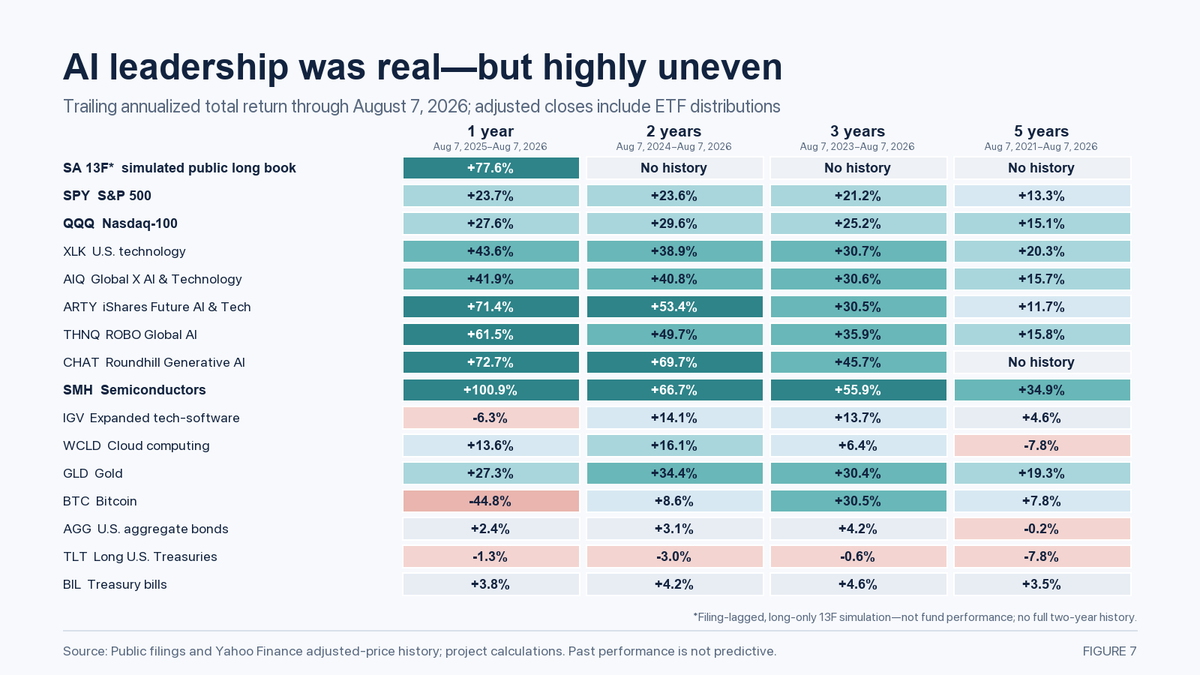
| Public series | 1 year annualized | 2 years annualized / SA since inception* | 3 years annualized | 5 years annualized |
|---|---|---|---|---|
| Situational Awareness LP — actual fund NAV | Not publicly reported | 2-year return not publicly reported; estimated ≈+445% cumulative since inception (approximately 21 months)* | Insufficient history | Insufficient history |
| Point-in-time 13F long-share simulation† | +77.6% | Insufficient public holdings history | Insufficient public holdings history | Insufficient public holdings history |
| SPY — S&P 500 | +23.7% | +23.6% | +21.2% | +13.3% |
| QQQ — Nasdaq-100 | +27.6% | +29.7% | +25.2% | +15.1% |
| XLK — U.S. technology | +43.6% | +38.9% | +30.7% | +20.3% |
| AIQ — broad AI | +41.9% | +40.8% | +30.6% | +15.7% |
| ARTY — future AI and technology | +71.4% | +53.4% | +30.5% | +11.7% |
| THNQ — artificial intelligence | +61.5% | +49.7% | +35.9% | +15.8% |
| CHAT — generative AI | +72.7% | +69.7% | +45.7% | Insufficient history |
| SMH — semiconductors | +100.9% | +66.7% | +55.9% | +34.9% |
| IGV — software | -6.3% | +14.1% | +13.7% | +4.6% |
| WCLD — cloud computing | +13.6% | +16.1% | +6.4% | -7.8% |
| GLD — gold | +27.3% | +34.4% | +30.4% | +19.3% |
| Bitcoin | -44.8% | +8.6% | +30.5% | +7.8% |
| AGG — aggregate bonds | +2.4% | +3.1% | +4.2% | -0.2% |
| TLT — long Treasuries | -1.3% | -3.0% | -0.6% | -7.8% |
| BIL — Treasury bills | +3.8% | +4.2% | +4.6% | +3.6% |
For Situational Awareness, “not publicly reported” is retained for actual trailing one- and two-year returns. Because the fund had only approximately 21 months of active history from the SEC-reported November 1, 2024 first-sale date through July 31, 2026, the two-year column additionally presents the estimated ≈+445% cumulative since-inception result. It is not annualized, is not an audited trailing two-year return and is derived from rounded reported milestones. The separate reported-performance panel retains the +47%, +439%, -67% and approximately +80% year-to-date figures. Transaction and counterparty narrative remains intentionally excluded, consistent with the article’s editorial and legal-risk scope.
†The one-year simulation begins on August 7, 2025 with the most recently public 13F long-share weights, then changes its holdings only after each subsequent filing became public. It uses adjusted public-market prices and excludes options, short positions, private assets, fees, financing, cash flows and undisclosed trades. It is a point-in-time reconstruction, not actual fund performance. A two-year version cannot be constructed without look-ahead bias because no Situational holdings were public at the August 7, 2024 start date.
The results support four conclusions.
First, the AI cycle produced genuine public-market outperformance. Semiconductors were the dominant winner across all four horizons.
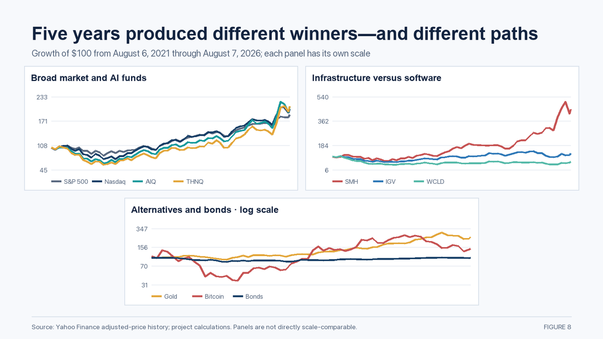
Second, “AI” was not one return stream. Broad AI funds, chip infrastructure, software, cloud companies and alternative assets behaved very differently. The five-year gap between SMH and WCLD was approximately 43 percentage points per year.
Third, a simple liquid semiconductor ETF captured much of the infrastructure upside without the financing, single-name, private-asset and operational risks of a concentrated hedge-fund structure. It still suffered high volatility and a 35.7% three-year maximum drawdown, so the ETF was not low risk—only operationally simpler.
Fourth, non-AI assets were not uniformly return-dilutive. Gold produced a 19.3% five-year annualized return and had far lower equity beta than the AI funds. Bonds disappointed over the period but could still provide collateral liquidity that a leveraged portfolio values differently from headline return.
Risk-adjusted comparison
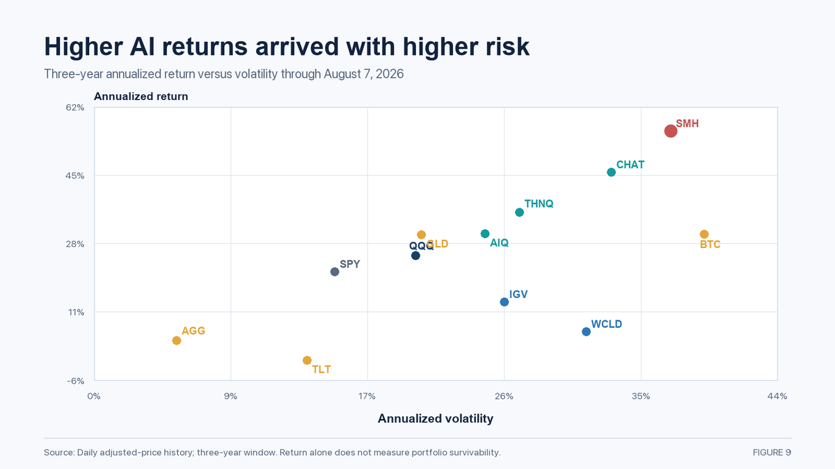
| Series | 3-year return | Volatility | Sharpe | Maximum drawdown | Beta to SPY |
|---|---|---|---|---|---|
| SPY | 21.2% | 15.4% | 1.06 | -18.8% | 1.00 |
| QQQ | 25.2% | 20.5% | 0.99 | -22.8% | 1.27 |
| AIQ | 30.6% | 25.0% | 1.03 | -26.4% | 1.43 |
| THNQ | 35.9% | 27.2% | 1.11 | -29.9% | 1.52 |
| CHAT | 45.7% | 33.0% | 1.18 | -31.3% | 1.74 |
| SMH | 55.9% | 36.8% | 1.28 | -35.7% | 1.93 |
| IGV | 13.7% | 26.2% | 0.46 | -36.6% | 1.24 |
| WCLD | 6.4% | 31.4% | 0.21 | -42.1% | 1.25 |
| GLD | 30.4% | 20.9% | 1.16 | -26.4% | 0.24 |
| Bitcoin | 30.5% | 39.0% | 0.54 | -53.1% | 1.02 |
| AGG | 4.2% | 5.3% | -0.04 | -5.0% | 0.07 |
| TLT | -0.6% | 13.6% | -0.33 | -14.8% | 0.13 |
Sharpe ratios use the BIL Treasury-bill ETF as a daily cash-return proxy. These are backward-looking estimates, not forecasts or published fund statistics.
The most revealing comparison is not SMH’s high return. It is the combination of a 1.93 market beta, 36.8% annualized volatility and a 35.7% drawdown. A portfolio levered four or five times cannot treat those characteristics as temporary noise. Even an asset with outstanding realized returns can be incompatible with the liability structure used to own it.
What the public ETFs cannot represent
No listed ETF is a clean market-price proxy for a private frontier-model developer. CHAT, AIQ, ARTY and THNQ hold public sponsors, suppliers and beneficiaries; they do not convert private-company valuations into daily returns. Private-company fundraising and valuation data therefore belong in a separate capital-formation analysis, not in the return table above.
Likewise, IGV and WCLD are broad software baskets. They illustrate how software and cloud exposure behaved, but they do not prove that every SaaS company was helped or harmed by a particular model release. Company-level outcomes depend on pricing power, distribution, seat exposure, inference cost, product velocity and whether AI expands usage or compresses margins.
PART 8 | CONCENTRATION VERSUS LEVERAGE
Was the problem concentration or leverage?
My answer is both—but they performed different roles.
| Portfolio structure | Likely result in a severe July-style reversal |
|---|---|
| Concentrated but unlevered | Very large drawdown, but the investor may retain the choice to hold or rebalance |
| Levered but genuinely diversified and liquid | Losses amplified, but smaller common-factor shock and easier liquidation may preserve control |
| Concentrated, high-beta, partly illiquid and 4×–5× gross | Greatly amplified drawdown and sharply reduced portfolio flexibility |
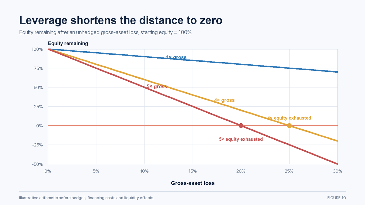
If $1 of equity controls $5 of gross assets, a 10% unhedged asset loss cuts the equity approximately in half. A 20% loss consumes it.
That is why leverage is central to the loss-amplification analysis.
But leverage alone does not explain why the asset book could move so much. The underlying shock came from:
- name concentration;
- common AI-capex exposure;
- high beta and volatility;
- crowded momentum;
- large positions relative to liquidity;
- short-side losses;
- and a possible deterioration in financing flexibility.
Drawdown recovery math
A 67% drawdown requires a 203% gain to return to the prior peak:
Required recovery = 1 / (1 - 0.67) - 1 = 203%
This is why being “still up for the year” does not make a 67% drawdown institutionally minor.
It can permanently reduce capital, investor confidence, financing capacity, employee retention, strategy flexibility and the manager’s ability to re-enter positions.
Success may have increased the risk
The fund reportedly gained 439% through June 30. Rapid gains and rapid inflows can create procyclical risk:
- larger dollar positions;
- increased borrowing capacity;
- more ownership concentration;
- worse exit capacity;
- and greater confidence in the recent regime.
If leverage rises with recent profits, the strategy becomes most exposed after its best performance.
PART 9 | WHAT THE PUBLIC EVIDENCE DOES NOT ESTABLISH
Public reporting described later changes involving the public-equity portfolio. This article does not analyze that activity or any participant in it.
The public record used here does not provide the complete terms, contemporaneous position file, internal communications or decision chronology. The article therefore draws no conclusion about the reasons, terms, decision process, market effects or subsequent economics of any specific transaction.
The quantitative analysis stops at observable security prices and clearly labeled public-holdings proxies. Event-window returns describe timing; they do not establish causation.
PART 10 | WHAT HISTORY CAN AND CANNOT TELL US
No historical episode is identical. The value comes from comparing mechanisms.
| Episode | What was genuinely compelling | Hidden common factor | Funding/liquidity problem | Lesson for AI portfolios |
|---|---|---|---|---|
| Dot-com bubble | The internet was transformative | Valuation, speculative growth and external capital | Capital markets closed for unprofitable companies | Correct technology thesis does not guarantee correct security or price |
| Housing credit | Housing assets appeared geographically diversified | Common underwriting and house-price factor | Long, opaque assets funded with unstable short-term liabilities | Many securities can become one correlated exposure |
| Asian currency crisis | High-growth economies attracted capital | Unhedged FX and confidence | Short-term foreign debt against longer-term domestic assets | A maturity mismatch can turn a solvency question into a liquidity run |
| LTCM | Relative-value relationships had economic logic | Correlations and convergence assumptions | High leverage met disappearing liquidity | Normal-regime correlations are not stress-regime correlations |
Dot-com: right technology, wrong price or company
The Federal Reserve’s 2001 market review described lofty technology valuations, sharp earnings reassessments and 27 days during 2000 when the Nasdaq moved at least 5%.
The internet did not fail.
Many investment structures did.
Today’s profitable hyperscalers are very different from revenue-free dot-coms. But private AI, marginal infrastructure developers and high-multiple suppliers can still experience the same gap between real technological progress and investor return.
Housing: apparent diversification can disappear
Mortgage pools looked diversified by borrower and geography. Common underwriting, leverage and reliance on continued refinancing made them far more correlated than historical models assumed.
Former Federal Reserve Chair Ben Bernanke later highlighted high leverage, unstable short-term funding and opaque instruments as core vulnerabilities.
The AI analogy is not that data centers equal subprime mortgages. They do not.
The analogy is that many different assets can depend on the same financing and demand assumptions.
Asian currency crisis: the sudden stop
The IMF’s review emphasized unhedged foreign-currency debt and short-term borrowing against longer-term assets.
When confidence changed, short-term funding conditions tightened before the underlying economies could adjust.
The AI-portfolio lesson is that a long-duration thesis can be vulnerable when financing conditions change much faster than the thesis horizon.
LTCM: liquidity is part of the position
LTCM’s trades were often based on sensible convergence relationships. During stress, spreads widened, correlations changed, and liquidity disappeared. The Federal Reserve’s history describes how leverage increased the fund’s vulnerability.
The important lesson is that liquidity is not an external detail.
Liquidity is part of the position. Financing is part of the position. Time is part of the position.
PART 11 | HOW PROFESSIONAL RISK TEAMS ANALYZE PORTFOLIOS
Professional research firms, asset managers and risk teams do not evaluate a portfolio using only total return or the number of holdings.
Core return and risk terminology
| Measure | Plain-English meaning | Why it matters here |
|---|---|---|
| Return | Change in NAV after fees and cash flows | A 13F basket return is not fund return |
| Alpha | Return unexplained by selected market/factor exposures | A large return generated by 4× sector beta may not be alpha |
| Beta | Sensitivity to a benchmark | The March long proxy’s short-window beta was approximately 4.08 to SPY and 2.71 to QQQ |
| Volatility | Dispersion of returns | The proxy’s April–August annualized volatility was approximately 85% |
| Sharpe ratio | Excess return per unit of total volatility | Can look exceptional during a short melt-up and fail to capture liquidity jumps |
| Sortino ratio | Return per unit of downside volatility | Better focused on negative outcomes but still historical |
| Maximum drawdown | Largest peak-to-trough loss | Directly connects risk to recovery math |
| Gross exposure | Absolute long plus absolute short/derivative-equivalent exposure divided by NAV | Measures balance-sheet scale |
| Net exposure | Long minus short exposure | Can hide risk if longs and shorts have different betas or factors |
| Beta-adjusted net | Long beta exposure minus short beta exposure | Better measure of market direction than dollar net |
| HHI / effective names | Name concentration and equivalent equal-weight count | Shows why 26 tickers behaved more like seven positions |
| Correlation/covariance | How positions move together | Correlation increased in the loss state |
| Value at Risk | Estimated loss threshold at a confidence level | Needs tail and liquidity context |
| Expected Shortfall | Average loss beyond the VaR threshold | More informative about severe tails |
| Marginal contribution to risk | How much each position adds to portfolio risk after correlation | Six positions generated most of the proxy loss |
| Days to liquidate | Time required to exit at a prudent share of market volume | Large ownership can turn a quoted price into an unrealistic exit price |
| Option Greeks | Delta, gamma, vega and theta | Underlier notional alone cannot describe the hedge |
What the daily risk report should show
An institutional AI portfolio should monitor:
- gross and net exposure;
- beta-adjusted net;
- name, theme and issuer limits;
- delta- and stress-adjusted derivatives;
- rolling and stressed correlations;
- principal-component concentration;
- expected shortfall and drawdown;
- liquidity days at normal and stressed volume;
- liquid collateral and financing headroom;
- private-asset collateral haircuts;
- borrow cost and short squeeze risk;
- option expiry and convexity;
- and a scenario in which financing requirements tighten simultaneously.
The general lesson is that leverage, concentration and insufficient liquidity preparation can interact rather than remain separate risks.
Governance matters
The person with the strongest conviction in a theme should not be the only person deciding whether the balance sheet survives.
An independent risk function should be able to:
- stop leverage from increasing after price gains;
- cap factor exposure across nominally different industries;
- require enough liquid collateral;
- distinguish an alpha short from a true hedge;
- reduce risk after a volatility or correlation regime change;
- and override a portfolio that cannot remain within its liquidity limits during stress.
This is not about eliminating conviction.
It is about preserving the ability to keep expressing conviction.
PART 12 | PRIVATE-MARKET AI EXPOSURE AND THE BROADER CAPITAL CYCLE
Publicly available information suggests that Situational Awareness has participated in private investments spanning several layers of the AI value chain. Because private-fund disclosures are limited, these exposures are better considered as broad industry groups rather than as a complete company-level portfolio.
| Private-market exposure group | Role in the AI value chain | Important information not available publicly |
|---|---|---|
| Frontier AI and model development | Development and training of advanced foundation models and AI systems | Entry valuation, ownership percentage, investment cost, preference terms, dilution and independently verified carrying value |
| Specialized compute and data-center infrastructure | Computing capacity, infrastructure and hosting for model training and inference | Fund commitment, debt and SPV structure, customer concentration, utilization, capital requirements and liquidity terms |
| AI semiconductor and systems development | Specialized processors, accelerators and supporting hardware | Investment valuation, ownership, manufacturing dependencies, commercialization risk, future funding requirements and dilution |
These categories are illustrative and may not represent the complete private portfolio. Public financing announcements can establish participation in selected transactions, but they generally do not disclose the information required to calculate the fund’s economic exposure or investment return.
The public record does not provide a reliable view of investment cost, ownership percentages, side letters, preferred rights, co-investment vehicles, debt arrangements, internal valuation policies or the amount of fund capital allocated to each private position. Consequently, the private portfolio cannot be reconstructed accurately or compared directly with public-market indices.
Private marks are not liquidity
A private company can be extremely valuable and still be unusable for an immediate liquidity need.
Private investments introduce:
- stale valuation risk;
- limited secondary liquidity;
- liquidation preferences;
- future dilution;
- customer and supplier concentration;
- multi-year time to exit;
- and collateral haircuts.
A hybrid public/private fund can have positive long-run NAV while facing immediate public-market financing stress.
AI venture capital is itself concentrated
The NVCA 2026 Yearbook reports that AI captured 65.4% of U.S. venture deal value in 2025. The five largest financings accounted for nearly $60 billion collectively.
Stanford’s 2026 AI Index estimates $285.88 billion of U.S. private AI investment in 2025.
That capital is funding real development.
It also creates portfolio questions:
- Are many investors exposed to the same small set of companies?
- How much demand is funded by investor capital rather than customer free cash flow?
- How much infrastructure is secured through debt, leases and special-purpose vehicles?
- What happens when a private financing window closes for twelve months?
- Which valuations assume a rapid IPO exit?
The application layer matters
Menlo Ventures estimates that enterprises spent $37 billion on generative AI in 2025, with $19 billion—more than half—at the application layer.
That is an important counterweight to a permanent “long infrastructure, short software” view.
Infrastructure enables AI.
Applications may capture much of the customer value.
Platforms may capture distribution.
Model providers may capture intelligence economics.
Power and chip providers may capture scarcity.
The dominant layer can rotate as the cycle develops.
PART 13 | A MORE SURVIVABLE AI PORTFOLIO FRAMEWORK
Again, this is not a recommended portfolio. It is an institutional risk thought experiment.
The first rule is that AI exposure should be a sleeve inside a broader portfolio—not the entire portfolio relabeled across multiple AI-adjacent industries.
There is no single correct AI portfolio. The structure should match the investor’s liabilities, liquidity, governance and ability to tolerate drawdowns.
Strategy structures worth comparing
| Structure | How it expresses AI | Principal advantage | Principal failure mode |
|---|---|---|---|
| Concentrated infrastructure | Direct positions in chips, power, memory, data centers and neoclouds | Strongest participation if capex keeps accelerating | One economic factor, high valuation and financing sensitivity |
| Core and satellite | Broad index core plus a limited AI sleeve | Keeps AI upside without making it the entire portfolio | Can feel disappointingly conservative during a melt-up |
| AI barbell | Profitable platforms and infrastructure on one side; T-bills and explicit protection on the other | Liquidity to rebalance after a shock | Cash drag and recurring hedge cost |
| Value-chain diversified | Infrastructure, platforms, applications and selected users | Participates if value capture rotates between layers | Still exposed to aggregate AI expectations and broad technology beta |
| Risk-balanced AI | Position sizes based on volatility and risk contribution rather than dollars | Prevents the most volatile names from dominating | Can underweight the strongest winners and relies on unstable correlations |
| Market-neutral relative value | Long preferred companies and short closely matched peers | Lower intended market and sector beta | Borrow, squeeze, basis and model risk; dollar neutrality is not factor neutrality |
| Option-defined exposure | Calls, call spreads or put-protected positions with preset loss budgets | Makes maximum premium or spread loss explicit | Timing, decay, volatility pricing and roll cost |
For many long-horizon investors, the most robust design is likely to resemble core and satellite or a value-chain portfolio with an explicit liquidity reserve. That is not because those structures maximize upside. It is because they reduce the probability that a single regime change determines the entire portfolio’s future.
An illustrative structure might limit AI to 20%–30% of total liquid NAV, depending on mandate and risk tolerance. The remaining portfolio would contain assets with different economic drivers.
Within the AI sleeve:
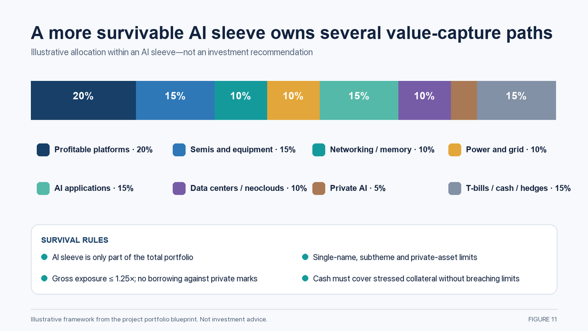
| AI sleeve | Illustrative weight | Role | Primary failure mode |
|---|---|---|---|
| Profitable platforms/hyperscalers | 20% | Cash-flow-funded AI and distribution optionality | Capex inefficiency, regulation, model commoditization |
| Semiconductors and equipment | 15% | Scarce compute and manufacturing | Inventory cycle, export controls, customer concentration |
| Networking, memory, storage and cooling | 10% | Non-accelerator bottlenecks | Capacity additions, pricing and substitution |
| Grid, generation and power equipment | 10% | Electricity and interconnection demand | Regulation, fuel, rates and project delays |
| AI applications and software | 15% | Customer monetization and productivity | Weak moats, platform bundling and seat compression |
| Data centers and neoclouds | 10% | Deployment and inference capacity | Debt, utilization, residual chip value, customer concentration |
| Private AI | 5% | Frontier access and convexity | Stale marks, dilution, technical displacement, no exit |
| T-bills, cash and explicit hedges | 15% | Collateral, rebalancing and tail protection | Cash drag in a melt-up |
Example hard limits
- AI sleeve: 25% target, 30% ceiling after appreciation.
- Single public company: 3% of total NAV; 5% absolute ceiling.
- Single AI subtheme: 8%–10% of total NAV.
- All private AI: 5% of total NAV; one private company: 1%.
- Gross exposure: 1.25× NAV maximum; normal target at or below 1.0×.
- No structural borrowing against private marks.
- Option premium at risk: 1%–2% of NAV per year.
- At least 90% of the public book exit-able in ten normal trading days using no more than 15% of expected daily volume.
- Cash/Treasury reserves sufficient for a severe twenty-trading-day liquidity event.
- Drawdown gates that reduce factor exposure before portfolio flexibility deteriorates.
These are examples for discussion, not universal risk limits.
Hedge the actual loss state
A short position is not automatically a hedge.
For an AI-infrastructure portfolio, more direct hedges may include:
- puts or put spreads on the actual semiconductor/data-center factor;
- index futures sized to beta-adjusted exposure;
- same-industry relative-value shorts matched on quality, duration and momentum;
- rate hedges for duration-sensitive projects;
- commodity hedges where power economics depend on fuel;
- and enough cash to avoid turning a temporary price decline into a loss of investment flexibility.
Keep two books:
- Hedge book: judged by how much tail loss it removes and what carry it costs.
- Alpha short book: judged independently on fundamentals, catalyst, borrow and squeeze risk.
Do not give an alpha short risk-reduction credit unless the covariance and stress scenarios support it.
Prepare for rotation
| Regime | Likely relative winners | Likely underweights | Portfolio response |
|---|---|---|---|
| Capex acceleration, easy credit | Chips, memory, neoclouds, data centers | Cash and defensives | Rebalance appreciation-created concentration |
| Capex acceleration, tight credit | Profitable platforms, equipment monopolies, contracted power | Levered neoclouds and speculative developers | Upgrade balance-sheet quality |
| Capex digestion, application monetization | Platforms, AI-native applications and software | Commodity compute and marginal capacity | Rotate toward revenue capture and free cash flow |
| Efficiency shock | Applications and low-cost inference | Highest-cost compute and marginal generation | Stress utilization and hardware residual values |
| Risk-off/credit closure | T-bills, cash-generative platforms and regulated assets | Negative-cash-flow, highly leveraged equities | Cut gross early and preserve dry powder |
Watch the cycle before price becomes the only signal
The most useful warning system combines fundamental, financing and market indicators.
| Warning category | Indicators to monitor | Why it matters |
|---|---|---|
| Hyperscaler demand | Capex guidance, accelerator orders, depreciation policy and free-cash-flow conversion | Tests whether the marginal infrastructure dollar is still growing |
| Lab economics | Revenue quality, inference cost, gross margin, customer concentration and funding runway | Separates usage growth from sustainable purchasing power |
| Capacity | GPU rental pricing, utilization, power reservations, construction delays and memory inventories | Detects whether scarcity is becoming overcapacity |
| Financing | Credit spreads, data-center debt terms, lease guarantees, collateral terms and equity issuance | Shows whether the buildout remains financeable |
| Market regime | Breadth, momentum, implied volatility, short interest and cross-asset correlation | Identifies crowding and a transition from differentiation to liquidation |
| Portfolio survival | Gross exposure, stressed collateral, days to liquidate and drawdown gates | Determines whether the investor retains control of the exit date |
No single indicator calls the top. The concern rises when demand revisions, weaker financing and deteriorating breadth occur together while portfolio leverage remains high.
Stress tests I would require
- 2000-style multiple compression: revenue grows, but terminal multiples fall 50% and unprofitable names fall 70%–90%.
- 2022-style rate shock: real yields rise 200 basis points and private financing closes for twelve months.
- Financing shock: collateral haircuts double while market liquidity falls 70%.
- Efficiency shock: compute per useful task falls faster than usage grows.
- Supply glut: memory, accelerator rental and equipment pricing fall together.
- Application capture: software and applications outperform infrastructure by 50 percentage points.
- Geopolitical supply shock: logic and memory supply are disrupted with price, volume and currency effects.
- Private-mark shock: private AI marks fall 50%, make no distributions for three years and receive zero collateral value.
The portfolio passes only if it can maintain required liquidity and remain within its risk limits.
A positive expected ten-year return is not enough.
PART 14 | WHAT WE MAY STILL BE MISSING
The public evidence is meaningful, but incomplete.
The portfolio changed after March
A May 2026 Schedule 13G disclosed 12.41 million Nebius shares. SK Hynix was a foreign position not covered by the U.S. 13F. Actual July weights may have differed materially from the March snapshot.
The puts may have produced substantial gains
Without strikes, expirations, premiums, deltas and daily trades, the result cannot be reconstructed from the filing.
Investor flows may have changed the balance sheet
Subscriptions, redemptions, fees and side-pocket terms can materially change NAV and liquidity independently of security returns.
The financing chronology is unavailable
Public data do not provide the portfolio’s complete financing terms or a decision-by-decision chronology. This article therefore draws no conclusion about how financing arrangements affected any specific transaction.
The private book may dominate the remaining economics
Private AI holdings may preserve enormous value. They can also experience valuation, dilution and liquidity risk. Both can be true.
The market move was broader than one fund
Semiconductors and AI infrastructure were already rotating. The public price record alone cannot attribute those market moves to any particular investor or transaction.
Scale may have been the hidden variable
A strategy that works at $1 billion can behave differently at $45 billion because ownership, market impact, staffing, financing complexity and liquidity capacity do not scale linearly.
These unknowns limit the precision of the P&L attribution.
They do not remove the visible structural vulnerability: concentration, leverage, volatility and liquidity were not independent risks.
CONCLUSION | BUILD THE FUTURE, BUT SURVIVE THE PATH
I remain positive about the long-term potential of AI.
I think Aschenbrenner’s broad view—that AI is an industrial, energy, semiconductor, infrastructure and geopolitical story, not only a software feature—was an important insight.
The portfolio lesson is different.
The future can arrive late.
It can arrive through different companies.
It can create more value for customers than suppliers.
It can shift from training to inference, from infrastructure to applications, from scarcity to overcapacity, and from equity-funded growth to credit-constrained consolidation.
A portfolio must survive all of those paths.
The deepest lesson I take from this case is:
The strength of a thesis should determine what you research. The downside and liquidity structure should determine how much you own.
The best AI portfolio may not be the one with the highest exposure to the most vivid forecast.
It may be the one that can remain invested when:
- the theme falls 50%;
- correlations go to one;
- software outperforms infrastructure;
- private markets close;
- financing conditions tighten;
- and the investment thesis needs three more years.
That is not a negative view of AI.
It is a positive view disciplined by portfolio survival.
AI may still be the dominant capital cycle of the decade. The investors who benefit most may be those who combine technological imagination with valuation, diversification, liquidity, independent risk control and patience.
Build the future. Finance it so you are still there when it arrives.
FINAL DISCLAIMER
This article is provided solely for educational, analytical and discussion purposes. It is based on public information that may be incomplete, delayed, revised or incorrect. All portfolio returns in the analysis are explicitly labeled public-market proxies and should not be treated as the performance of Situational Awareness LP or any investor.
Nothing in the article is intended as an accusation, criticism or adverse characterization of Leopold Aschenbrenner, Situational Awareness LP, their employees, investors, portfolio companies or the AI industry. Nothing suggests misconduct or wrongdoing. The discussion evaluates general portfolio-construction mechanisms that can apply to any concentrated strategy.
Nothing is investment, legal, tax or accounting advice. The article does not recommend any security, fund, position, allocation or transaction. Readers should conduct independent research and consult appropriately qualified professionals before making financial decisions.
METHODOLOGY AND PRIMARY SOURCES
Original thesis and fund description
- Leopold Aschenbrenner, Situational Awareness: The Decade Ahead, June 2024.
- Situational Awareness LP and About.
Regulatory sources
- Situational Awareness Partners LP Form D/A, reporting November 1, 2024 as the date of first sale.
- 2025 Q1 Form 13F
- 2025 Q2 Form 13F
- 2025 Q3 Form 13F
- 2025 Q4 Form 13F
- 2026 Q1 Form 13F
- SEC Form 13F FAQ
- Nebius Schedule 13G, May 27, 2026.
- SEC Investment Adviser Public Disclosure
Reported fund-performance sources
- Fortune via Yahoo Finance, profile reporting a 47% net return in the first half of 2025.
- Yahoo Finance, reporting a 439% net return through June 30, 2026, attributed to the July 24 investor letter.
- Wall Street Journal, “His Wedding Guests Were Arriving—Just as His $45 Billion Fund Was Falling Apart”.
- Wall Street Journal, “Situational Awareness Down 67% in July in AI Stock Rout”.
- Cinco Días, reporting the 439% first-half 2026 and 1,551% since-inception figures.
AI, power and venture-market context
- IEA, Energy and AI.
- Stanford HAI, 2026 AI Index — Economy.
- NVCA 2026 Yearbook.
- Menlo Ventures, The State of Generative AI in the Enterprise 2025.
Public AI benchmark definitions
- Global X, AIQ — Artificial Intelligence & Technology ETF.
- iShares, ARTY — Future AI & Tech ETF.
- ROBO Global, THNQ — Artificial Intelligence ETF.
- Roundhill, CHAT — Generative AI & Technology ETF.
- VanEck, SMH — Semiconductor ETF.
- iShares, IGV — Expanded Tech-Software Sector ETF.
- WisdomTree, WCLD — Cloud Computing Fund.
Historical and risk-management sources
- Federal Reserve History: LTCM near-failure.
- Federal Reserve: Archegos and leverage.
- Federal Reserve: Great Recession.
- IMF: The Asian Financial Crisis—What Have We Learned?.
- CFA Institute: Portfolio Mathematics.
Market-data methodology
Daily adjusted closes were retained from Yahoo Finance’s chart endpoint through August 7, 2026. ETF adjusted prices include distributions where supplied by the data source; Bitcoin uses the BTC-USD spot series. Trailing returns are annualized over the actual elapsed calendar period. Volatility, beta, alpha, correlation, Sharpe and Sortino estimates use daily returns; Sharpe and Sortino use BIL as the cash-return proxy. Maximum drawdown is calculated from the daily adjusted-price path.
The long-book comparison uses March 31 long-share weights as a buy-and-hold proxy from March 31 through August 7. It excludes short stock, options, private investments, leverage, financing costs, fees, subscriptions, redemptions and trading after the filing date. It is not actual or estimated fund NAV performance.
The five-year public comparison begins with the last available adjusted close on or before August 7, 2021. CHAT is marked unavailable for the five-year window because it began trading in May 2023. No current-holdings backcast is presented because that would introduce look-ahead and survivorship bias. SK Hynix returns elsewhere in the event analysis are local-currency unless stated otherwise. No basket is represented as actual fund performance.
The full reproducible research project—including normalized filings, calculations, holdings inventory, technical analysis and portfolio blueprint—is maintained separately from the publishable article.
APPENDIX | MARCH 31, 2026 DISCLOSED POSITION INVENTORY
Long shares and convertibles
| Ticker | Issuer | SEC value | Theme |
|---|---|---|---|
| BE | Bloom Energy | $878.7M | Power generation |
| SNDK | Sandisk | $724.4M | Memory/storage |
| CRWV | CoreWeave | $556.1M | AI neocloud |
| IREN | IREN | $401.0M | Miner-to-AI/data centers |
| CORZ | Core Scientific | $389.1M | Miner-to-AI/data centers |
| APLD | Applied Digital | $320.0M | AI data centers |
| RIOT | Riot Platforms | $142.2M | Miner-to-AI/data centers |
| CLSK | CleanSpark | $104.5M | Miner-to-AI/data centers |
| SEI | Solaris Energy Infrastructure | $62.5M | Power equipment |
| TE | T1 Energy | $43.9M | Power generation |
| KEEL | Keel Infrastructure, formerly Bitfarms | $38.8M | Miner-to-AI/data centers |
| BTDR | Bitdeer Technologies | $29.8M | Miner-to-AI/data centers |
| PSIX | Power Solutions International | $26.3M | Power equipment |
| WYFI | WhiteFiber | $20.9M | AI data centers |
| AMD | Advanced Micro Devices | $20.2M | Semiconductors |
| BW | Babcock & Wilcox | $19.9M | Power equipment |
| SHAZ | SharonAI Holdings | $18.1M | AI neocloud |
| PUMP | ProPetro | $13.1M | Energy services |
| SMH | VanEck Semiconductor ETF | $10.3M | Semiconductors |
| INTC | Intel | $8.9M | Semiconductors |
| TSM | TSMC | $7.6M | Semiconductors |
| HIVE | HIVE Digital | $6.4M | Miner-to-AI/data centers |
| ASML | ASML | $6.1M | Semiconductor equipment |
| MU | Micron Technology | $5.9M | Memory semiconductors |
| GLW | Corning | $0.7M | Optical networking |
| NVDA | Nvidia | $0.5M | Semiconductors |
| Total | $3.856B |
Calls — value of underlying shares, not option premium
| Ticker | Underlier value | Underlying shares |
|---|---|---|
| MU | $422.3M | 1,250,000 |
| SNDK | $388.8M | 611,900 |
| TSM | $354.8M | 1,050,000 |
| CRWV | $140.6M | 1,814,500 |
| BE | $55.3M | 408,500 |
| Total | $1.362B |
Puts — value of underlying shares, not option premium
| Ticker | Underlier value | Underlying shares |
|---|---|---|
| SMH | $2.043B | 5,327,900 |
| NVDA | $1.568B | 8,992,300 |
| ORCL | $1.073B | 7,293,000 |
| AVGO | $1.006B | 3,251,100 |
| AMD | $969.2M | 4,764,100 |
| MU | $583.7M | 1,727,700 |
| TSM | $535.1M | 1,583,400 |
| ASML | $494.1M | 374,100 |
| INTC | $159.1M | 3,605,400 |
| GLW | $21.0M | 154,600 |
| INFY | $6.8M | 500,000 |
| Total | $8.459B |
End of article.